Through information bottleneck method, we know the goal of a learning system is to minimize $I(X;T)$ to encourage maximal compression which can be narrowly interpreted as feature selection, or the gathering of the minimum sufficient statistics: $Y - X - S(X) - T(X)$¹ so that $I(X; Y) = I(S(X); Y) = I(T(X); Y)$. The other objective of an optimal learning system, according to Tishby, is to encourage the extracted reprerensetation to share its statistical distribution to the label space $Y$ by maximizing $I(Y; T)$.

\[\begin{equation*} \begin{aligned} & \text{minimize} & & I(X;T) \\ & \text{maximize} & & I(Y;T) \\ \end{aligned} \end{equation*} \tag{1} \label{original}\]

We can reformulate to allow this to have a soft objective as:

\[\begin{equation*} \begin{aligned} \min\limits_{p(t|x), p(y|t), p(t)} \{I(X;T) - \beta I(T;Y)\} \\ \end{aligned} \end{equation*} \tag{2} \label{info_bottleneck}\]

In fact, Tishby² has shown that under an theooptimal algorithm: The Blahut–Arimoto algorithm, the problem can be solved exactly. However, Blahut-Arimoto algorithm cannot be computed exactly with integration, so we have to approximate both $I(X; T)$ and $I(Y; T)$.

Preliminary studies have shown a simple way to approximate an upper bound of $I(X; T) - \beta I(T; Y)$ by using the non-negativity of mutual information for continuous random variables³. Alemi, et al has shown that in order to apply this principle to supervised learning, beyond rate distortion theory or compression, we want to be lenient to the rate of compression but be demanding on the mutual information between hidden representation and label, thus recasting the equation to be $\beta I(X;T) - I(T; Y)$.

We can expand each terms out, but for now we should focus on $I(T; Y)$, since this is the goal of learning:

\[I(T;Y) = \int p(y, t) \log \frac{p(y \vert t)}{p(y)} dy dt\]

The difficult part is to evaluate $p(y\vert t)$, and we use a variational approximation to this value. With an understanding that the bound can be arbitrarily loose, and with monte carlo sampling, Alemi et al derived that $I(X; T) \leq \mathrm{KL}[p(T \vert X), r(T)]$, with $r$ being an arbitrary distribution: spherical gaussian $\mathcal{N} \sim (0, I)$. And $-I(Y;T) \leq \mathbb{E}_{\epsilon \sim p(\epsilon)}[-\log q(Y \vert f(X, \epsilon))]$ where $q(Y \vert f(X, \epsilon))$ is our model.

Information Bottleneck (IB) principle assumes markov chain to be $Y - X - \hat{X}$. We can naively extend this to multilayer neural network $Y - X - h_1 - h_2 - … - h_n - \hat{X}$. And formulate our IB training objective as $I(X; h_1, …, h_n) - \beta I(Y; h_1, …, h_n)$. However, with simple deduction we can show that:

\[\begin{equation*} \begin{aligned} I(h_1, h_2 ; X) &= H(X) - H(h_1, h_2) \\ &= H(X) - H(h_2 \vert h_1) - H(h_1) \\ & = H(X) - H(h_1) \text{ with } X - h_1 - h_2 \\ & = I(X; h_1) \end{aligned} \end{equation*} \tag{3} \label{3}\]

This means we can only treat the output of a neural network as a random variable and we do not need intermediate stochastic representation if our algorithm is optimal.

This is not the only problem with this formulation. Think about $I(Y; T_i)$ term, if we expand it out as before, we will need to evaluate $p(Y \vert T_i)$, since it is a markov-chain:

\[\begin{equation} \begin{aligned} p(y\vert t_i) &= \int_{t_{1}...t_{n}} q(y \vert x, t_{n}...t_{i+1}, t_i,...,t_1)\mathrm{d}t \\ \end{aligned} \end{equation}\]

We can only calculate this probability density function when we integrate out all the other intermediate layers. This shows that in order to know each layer’s contribution to predicting the label, we need to factor out alll other layers. This is as intractable as it gets.

In order to circumvent this, we can learn from Shwartz-Ziv², who used a special way to measure the mutual information between each layer and the label $I(Y; T_i)$ using the following markov chain : $Y - X - T_i$. As for the compression part of IB principle $I(X; T_i)$, instead of approximating this quantity directly, we can use the successive compression rate defined as: $X - T_{i-1} - T_{i}$, and we measure $I(X; T_1)$ and $I(T_{i-1}; T_{i})$.

Thus we are able to reformulate the cost for a multi-layer stochastic neural network as:

\[L_{MIB} = [\sum_{i=1}^n I(Y; T_i)] + I(X;T_1) + \sum_{i=2}^n I(T_{i-1}; T_i)\]

This is equivalent to create sub-networks and add the $L_2$ norm of each layer to the cost (this term is equivalent to the KL divergence between layers and a spherical gaussian distribution).

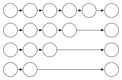
This is similar to the style of stochastic depth network (SDN)⁴, but in a more principled way. We encourage each layer to maximally compress $X$ and maximally increase the chance of predicting the correct label. This is quite different form the architecture of DenseNet⁵, which is applying residual connections between earlier layers and later layers.

Now we bridge the gap between a normal feedforward neural network and recurrent neural network. If we follow Yarin Gal’s derivation ⁶⁷, we can realize dropout is a special type of Bayesian approximation with tighter bounds than the reparameterization trick. Thus recurrent dropout, where dropout is applied to recurrent connections, can be seen as that recurrent hidden states in RNN being stochastic layers, without the need of adding a stochastic layer on top of a deterministic layer, which is what has been proposed by Fraccaro et al ⁸.

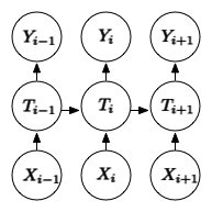
With recent regularization techniques such as Zoneout ⁹, we can see the essence of it being forcing previous hidden state to predict the current timestep’s outcome. Using what we have derived in information bottleneck objective, we can see it as $I(Y_i; T_{i-1})$, so Zoneout does not link to bayesian approximation like other dropout methods would, but it does link to mutual information-based training objective, thus one can argue whether the stochasticity of Zoneout is needed or not. We can formulate a training objective for RNN more deterministically:

\[L_{RNN} = [\sum_{i=1}^n I(Y; T_i)] + [\sum_{i=1}^n\sum_{s=1}^k I(Y_{i+s};T_i)] + I(X;T_1) + \sum_{i=2}^n I(T_{i-1}; T_i)\]

This formulation is equivalent to Zoneout when applied stochastically with slight modification. Intuitively, it will help the current hidden states to extract information that’s more relevant to the future.

Footnotes