Preface

This is an article providing another perspective on understanding Lagrangian and dual problem. These two topics are essential to convex and non-convex optimization. Since it is a blog post, the proper background to understand this article is kept rather low. If you need to brush up on convex knowledge, or wish to be introduced to the subject, there is a handout from Stanford CS229 website, and it’s written in a very concise and clear way: Convex Optimization (I) and Convex Optimization (II). However, you don’t need to understand convex sets and functions in order to follow this post. If you are like me, who took Stanford EE364A, then you might find this post more interesting. The post randomly jumps between Chapter 5, Chapter 10, and 11 in the book (Convex Optimization book by Stephen Boyd), but mostly focus on presenting Chapter 5. This post is also inspired by an office hour conversation with Nicholas Moehle.

Lagrangian

In convex optimization, unlike other fields of machine learning, we can add constraints. Convex problems have a form of the following:

\begin{equation*}
\begin{aligned}
& \text{minimize}
& & f_0(x) \\
& \text{subject to}
& & f_i(x) \leq 0, \; i = 1, \ldots, m. \\
&
& & h_i(x) = 0, \; i = 1, \ldots, p.
\end{aligned}
\end{equation*}

We define $f_i(x)​$ being convex functions, and $h_i(x)​$ being affine functions. If you are familiar with convex optimization or other optimization problem, this formula should look familar. The constraints listed under subject to are considered hard constraints, and those constraints do not normally appear in traditonal machine learning cost functions. One way to distinguish them is that, cost functions in Machine Learning does not need to have a realistic meaning (objective can be an abstract measurement of progress), where in convex optimization, objective is something you want to find (like how much fuel the rocket will need).

However, it has been quite difficult to optimize with these hard constraints. Typical methods include solving for a Newton step:

\begin{equation*}
\begin{bmatrix}
    \nabla^2f(x)  & A \\
    A & 0
  \end{bmatrix}
    \begin{bmatrix}
    \Delta x_{nt} \\
    w
  \end{bmatrix} =
  \begin{bmatrix}
    - \nabla f(x) \\
    0
  \end{bmatrix}
\end{equation*}

Solving for $\Delta x_{nt}$ and we get our central-path (feasible) Newton method of satisfying equality constraint as well as optimizing our overall objective. As to why it has such effect, refer to the book.

As to satisfy the inequality constraint, we can use barrier method, which adds the inequality constraints as a logarithmic barrier, so instead of optimizing the original problem, we can have:

\begin{equation*}
\begin{aligned}
& \text{minimize}
& & f_0(x) - (1/t) \sum_{i=1}^m \text{log}(-f_i) \\
& \text{subject to}
& & h_i(x) = 0, \; i = 1, \ldots, p.
\end{aligned}
\end{equation*}

The logarithmic barrier punishes the objective logarithmically when it’s approaching 0 from the negative side.

So what do those two “implementation” details have to do with Lagrangian? The reason is simple: Lagrangian is simply a way, not unlike equality Newton step or barrier method, to incoroporate constraints into the overall objective. It turns the hard constraints into soft constraints. Soft constraints that you (or the optimization) can violate.

Let’s look back to the first equation: we can formulate its Lagrangian as:

\begin{equation*}
L(x, \lambda, \nu) = f_0(x) + \sum_{i=1}^m \lambda_i f_i(x) + \sum_{i=1}^p \nu_i h_i(x)
\end{equation*}

Now it’s as if we are telling the God of optimization that, you can go ahead and violate our constraints as much as you can, and we are going to introduce two new variables $\lambda$ and $\nu$ to help you do that. These two variables are called dual variables. $\lambda$ is referred as inequality constraint dual variable, and not surprisingly $\nu$ is the equality constraint dual variable.

Dual Problem

After all these long and tedious definition of things (hopefully you aren’t too bored with them), we get to one last bit of information: dual problem. We can form a dual problem from the Lagrangian. What is a dual problem? Dual problem, simply put, is like you looking into the mirror. It’s you in the mirror, but the image is flipped. A deeper interpretation of dual problem is that it allows us to explore the effects of constraints on our original objective. Keep in mind that by forming Lagrangian, we allow the constraints to be soft, to add artibitrary large or small “penalty” to the original objective, but how would these constraints add penalization to the objective? dual variables provide the answer.

We first must get rid of the effect of $x$. Since we want to minimize the new objective (the Lagrangian), we can use the operator inf, it can give us the minimum value of the function over a chosen variable, and in here we choose $x$:

\begin{equation*}
g(\lambda, \nu) = \inf_{x \in D} L(x, \lambda, \nu) = \inf_{x \in D} \Big(f_0(x) + \sum_{i=1}^m \lambda_i f_i(x) + \sum_{i=1}^p \nu_i h_i(x) \Big)
\end{equation*}

By doing this, we reduce the first term $f_0(x)$, $f_i(x)$, and $h_i(x)$ to constants, and the infimum over a family of affine functions is a concave function (go through chapter 2 of the convex book for more details on this). Thus our dual objective is concave. Then we can quite awesomely form the following dual problem:

\begin{equation*}
\begin{aligned}
& \text{maximize}
& & g(\lambda, \nu) \\
& \text{subject to}
& & \lambda \succeq 0
\end{aligned}
\end{equation*}

A nicer understanding of this is that: by fixing $x$ (we shall now call it primal variable out of no reason…it’s actually to draw contrast to dual variables), we are driving the Lagrangian’s value down (as well as $f_0(x)$’s value), however, we must be violating constraints! So now, maybe it’s the time for the constraints to punish our objective, and we want the penalty to be as high as possible. Thus, by maximizing $g(\lambda, \nu)$, we can figure out a set of values for $\lambda$ and $\nu$ that will make the penalty as large as possible for the Lagrangian objective, hence the maximizing over $\lambda$ and $\nu$ on function $g$.

Geometric Analysis of Lagrangian

Now we can start our geometric interpretation of the Lagrangian. The problem rises when we alter the primal problem to form the lagrangian. We repeatedly ask ourself this question: does the newly formed Lagrangian become different from the primal problem in any way? If so, how can we avoid such primal-dual discordance by adding constraints? (Spoiler alert, these constraints become the famous KKT conditions).

We begin with the simplest example (as many explaination would start). You can easily extend them (mathematically, and mentally) to more complex problems. We first assume the simplest convex optimization problem, and we start with one equality constraint.

\begin{equation*}
\begin{aligned}
& \text{minimize}
& & f(x) \\
& \text{subject to}
& & h(x) = 0
\end{aligned}
\end{equation*}

We form the following Lagrangian: $L(x, \nu) = f(x) + \nu h(x)$. Notice the condition of optimality for the original problem is when $\nabla f(x) = 0$, and the optimality condition for the new Lagrangian is seemingly changed: $\nabla f(x) + \nu \nabla h(x) = 0$. We ask the question: will the change in optimality condition affect us from reaching the same goal (objective) as the original objective?

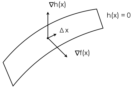
From the Lagrangian optimality condition, we can easily get $\nabla f(x) = -\nu \nabla h(x)$. Assume our final udpate to $x$ is $\Delta x$, meaning we move from our curent position $x$ to $x + \Delta x$, then in order to stay on the plane, $\Delta x$ must be orthogonal to the gradient vector of the plane ($h(x) = 0$), thus we get $\Delta x^T \nabla h(x) = 0$, and $\Delta x^T \nabla f(x) < 0$. Keep doing this, eventually, at the optimality point, we naturally have two gradient vectors being parallel (or anti-parallel, meaning pointing at different directions) becoming the end result when optimal solution is found. Notice we don’t require $\nabla f(x)$ and $\nabla h(x)$ to point at different directions, meaning $\nu$ doesn’t need to be positive or negative. Per our analysis, Lagrangian optimal condition captured what we would have wanted in the primal problem very nicely, we don’t need to add other constraints/conditions.

We get slightly more interesting result from examining the inequality constraint case. We can see the rise of KKT conditions and complementary slackness (two concepts that are often hard to grasp as first-timers) from the seemingly discordance between the original and Lagrangian optimality conditions.

\begin{equation*}
\begin{aligned}
& \text{minimize}
& & f(x) \\
& \text{subject to}
& & g(x) \leq 0
\end{aligned}
\end{equation*}

We formulate the simplest convex problem with one inequality constraint. The Lagrangian is $L(x, \lambda) = f(x) + \lambda g(x)$. The optimality condition for Lagrangian is $\nabla f(x) + \lambda \nabla g(x) = 0$. Now this case is slightly different from the equality case. We should first take a look at an illustration:

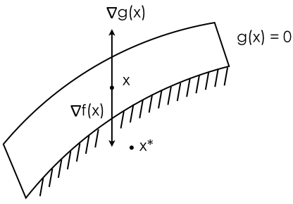
The shaded area including the surface when $g(x) = 0$ are the regions $x$ is allowed to be, satisfying our constraint. Like before, we can slightly reformulate the optimality condition to be: $\nabla f(x) = - \lambda \nabla g(x)$. We consider two cases. First, when $x$ is on the surface of $g(x) = 0$, meaning $x$ is on the boundary condition. When this is the case, it can only happen if $\nabla f(x)$ and $\nabla g(x)$ are pointing at opposite directions (notice gradient vector always points at the direction that increases function values), our desired direction is $-\nabla f(x)$. If not, meaning $\nabla f(x)$ and $\nabla g(x)$ are pointing at the same direction, all we need to do is to go to direction $-\nabla f(x)$, and we will decrease primal objective value as well as decreasing the value of $g(x)$, staying within $g(x) \leq 0$. To conclude, in order to have inequality constraint working, we must specify $\lambda > 0$.

Now we consider a second case, when $x$ is at $x^*$ position (below constraint surface). If the inequality constraint is satisfied, it should be effectively removed from the lagrangian equation, so that we are only optimizing under the primal optimal condition: $\nabla f(x) = 0$, thus $\lambda = 0$.

This is normally called “complementary slackness”, if $g(x) = 0$, then $\lambda > 0$, like our first case, and if $g(x) < 0$, then $\lambda = 0$, like our second case.

Now we are free to use what we have analyzed before, the conditions that will keep primal objective and Lagrangian the same:

1. Primal constraints: $f_i(x) \leq 0, i=1,…,m$, $h_i(x) = 0, i=1,…,p$
2. Dual constraints: $\lambda \succeq 0$
3. Complementary Slackness: $\lambda_i f_i(x) = 0, i =1,…,m $
4. Gradient of Lagnragian w.r.t $x$ vanishes: $\nabla f_0(x) + \sum_{i=1}^m \lambda_i \nabla f_i(x) + \sum_{i=1}^p \nu_i \nabla h_i(x) = 0$

These are also known as the KKT conditions. As we have pointed out before, if these conditions are satisfied, then Lagrangian and the primal problem are equivalent, meaning the primal problem has strong duality (refer to the book for more details).

Another fun fact is that, dual variables $\lambda$ and $\nu$, if KKT conditions are satisfied, (or if the primal problem has strong duality), then the dual variables are Lagrange multipliers.

Sensitivity Analysis

At last, we briefly mention sensitivity analysis. This portion was presented in a very confusing manner from the book (including powerpoint slides). If we take derivative of the Lagrangian with respect to the constraint:

\begin{equation*}
\lambda_i = - \frac{\partial g(\lambda^\star, \nu^\star)}{\partial f_i}
\text{,     }
\nu_i = - \frac{\partial g(\lambda^\star, \nu^\star)}{\partial h_i}
\end{equation*}

Notice that we are taking derivative of $g(\lambda^\star, \nu^\star)$. So the dual variable is the partial derivative of dual objective with respect to the constraints. Based on what we’ve learned from the last section, it’s not too difficult to reason that if $\lambda_i = 0$, the $i$ th inequality constraint is not constraining the objective. The larger $\lambda$ or $\nu$ is, the more constraining such constraint will be, a small change to tighten the constraint will cause a negative effect on the overall objective.

Dual variable $\lambda$ and $\nu$ are also known as shadow prices in economics.

Conclusion

This is the geometric intuition that slowly builds up the complementary slackness and the KKT condition. On first sight, KKT condition could be very daunting or confusing, same with complementary slackness. But a nice and solid grasp on directional gradient vectors will help provide a much cleaner understanding.